Creating Polygon Files

A common preprocessing step prior to running a Maha Multics simulation is to create polygon files defining boundary conditions. This section describes how to create geometry with the mahautils.shapes module and write polygon files with the mahautils.multics.PolygonFile class.

Note

For more details on the format of polygon files, refer to the Polygon File Format page.

Tutorial Geometry

For this tutorial, we will create a polygon file for a hypothetical case depicted below. Note that this geometry is not representative of a real pump; it is purely for demonstration purposes.

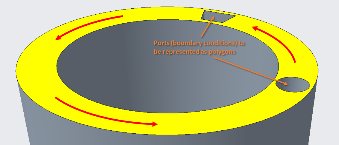
In this hypothetical example, the yellow surface is intended to represent a lubricating film, and the indicated ports are locations where polygons need to be defined so that constant-pressure boundary conditions can be imposed. Two shapes need to be captured: (1) a trapezoid and (2) a circle. In addition, notice that as indicated by the red arrows, the entire geometry rotates, so the polygon file needs to incorporate this motion.

The figure below shows a dimensioned view of the geometry and coordinate system which will be used in the remainder of the tutorial.

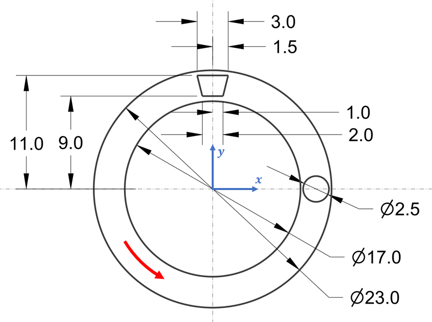
For this tutorial, we will assume that all dimensions are in millimeters.

Setup

To begin, open a Python terminal and import the classes from the MahaUtils package that will be used in this tutorial:

>>> from mahautils.multics import PolygonFile
>>> from mahautils.shapes import Circle, Layer, Polygon

Note that we could have imported the entire MahaUtils package (e.g., import mahautils), but importing specific classes only will make the tutorial code simpler and easier to understand.

Creating the Geometry

General Concepts

The intention of the mahautils.shapes package is to function similar to a graphics editor such as Inkscape. Individual shapes (circles, points, etc.) can be defined, and to aid in organizing complex geometry, shapes can be grouped in layers and layers can be grouped in a canvas.

Sometimes, it may be desirable to include construction geometry. This can be specified by setting the mahautils.shapes.Shape2D.construction property to True, and it signifies that the geometry should be included for visualization purposes, but it is only for reference and should not be written into a polygon file. For instance, this can be useful for defining the outer perimeter of the sealing land or hidden geometry.

Defining Geometry at Initial Position

Let’s first see how to define the port geometry in the initial position shown above. There are several shapes that need to be defined, so first create a mahautils.shapes.Layer to store them, optionally choosing the color to use when plotting the layer:

>>> layer_t0 = Layer(color='purple')

Two shapes need to be created to represent the ports: (1) a circle and (2) a trapezoid. These shapes can be created with the mahautils.shapes.Circle and mahautils.shapes.Polygon classes, respectfully, using the geometry shown in the previous diagrams:

>>> circle = Circle(center=(10, 0), diameter=2.5, units='mm',
...                 default_num_coordinates=100)
>>> trapezoid = Polygon(vertices=[[1, 9], [1.5, 11], [-1.5, 11], [-1, 9]],
...                     units='mm')

A few things to notice about these definitions:

• Units were specified with the units keyword argument. The commands above would still have worked even if we omitted this argument, but this would cause issues later when writing the polygon file.

• When plotting shapes with the mahautils.shapes package, the shapes are discretized into discrete points for plotting. The default_num_coordinates argument controls how many points are used to discretize the circle. However, it is not required for the trapezoid since a finite number of vertices were explicitly specified.

It can also be helpful to define construction geometry such as the inner and outer radii of the sealing land to provide a reference in visualization plots. Such geometry can be created with:

>>> circle_inner = Circle(center=(0, 0), diameter=17, units='mm',
...                       default_num_coordinates=100, construction=True)
>>> circle_outer = Circle(center=(0, 0), diameter=23, units='mm',
...                       default_num_coordinates=100, construction=True)

Now, we need to add all the shapes we created to the layer. The mahautils.shapes.Layer class functions the same way as a Python list, so any of the methods for modifying Python lists can be applied to the layer. For instance, we can extend the layer with the previously created shapes:

>>> layer_t0.extend([circle, trapezoid, circle_inner, circle_outer])

Finally, we can visualize the geometry we just set up using the mahautils.shapes.Layer.plot() method:

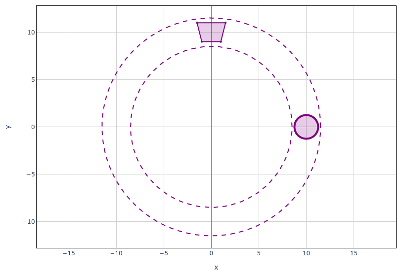
>>> layer_t0.plot()  

Running this should open a browser and show a figure similar to:

Defining Rotated Geometry

So far, we have created a layer with our desired geometry at the initial position However, as mentioned previously, the port geometry rotates. To include such rotating geometry in a polygon file, we need to generate layers with the rotated geometry for an arbitrary rotation angle.

One option to handle rotating geometry is to manually calculate the position of each shape for every rotation angle. However, this is fairly tedious and error-prone. A simpler approach is that since we have already defined the desired geometry, we can rotate it using the mahautils.shapes.Layer.rotate() method.

For instance, one way to implement this is to create a function that generates a new mahautils.shapes.Layer instance by rotating the geometry defined in the previous section:

>>> def layer_at_angle(angle, angle_units):
...     layer = Layer(color='purple')
...
...     layer.append(Circle(center=(10, 0), diameter=2.5, units='mm',
...                         default_num_coordinates=100))
...     layer.append(Polygon(vertices=[[1, 9], [1.5, 11], [-1.5, 11], [-1, 9]],
...                          units='mm'))
...
...     layer.append(Circle(center=(0, 0), diameter=17, units='mm',
...                         default_num_coordinates=100, construction=True))
...     layer.append(Circle(center=(0, 0), diameter=23, units='mm',
...                         default_num_coordinates=100, construction=True))
...
...     layer.rotate(center=(0, 0), angle=angle, angle_units=angle_units)
...
...     return layer

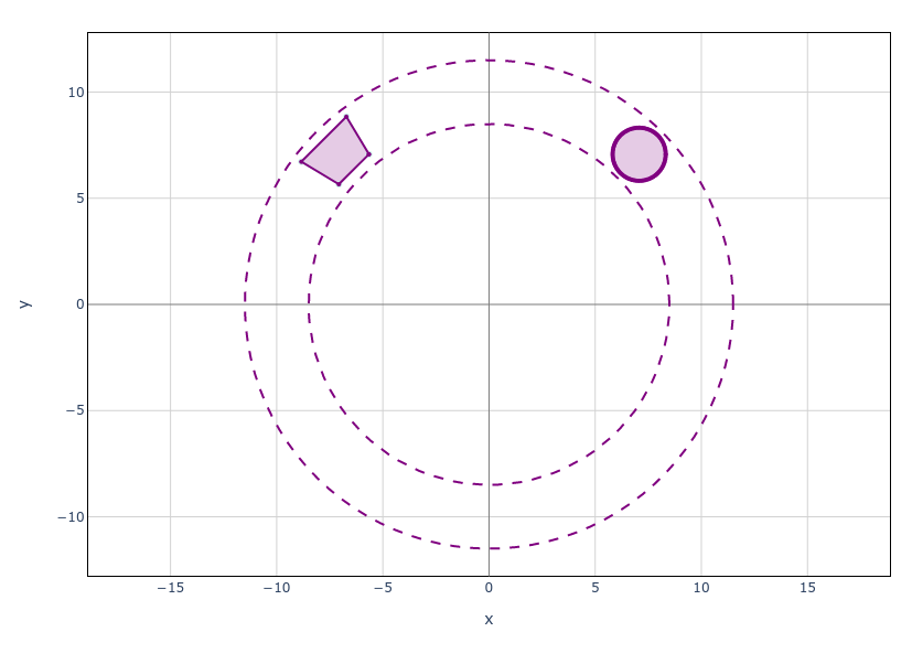
Now, we should be able to generate the geometry rotated to any angle. For instance, to plot the geometry at \(45^\circ\), run:

>>> layer_at_angle(45, 'deg').plot()  

This should generate a plot similar to:

Creating the Polygon File

So far, we have focused on setting up the geometry that we will store in the polygon file, and we have created a function layer_at_angle() which generates a mahautils.shapes.Layer containing the port geometry rotated to any angle. In this section, we will see how to save these data as a polygon file.

General Properties

First, begin by initializing a mahautils.multics.PolygonFile object:

>>> polygon_file = PolygonFile()

Next, there are a few general parameters which need to be defined. We want points inside of either port to be considered boundary conditions, so set:

>>> polygon_file.polygon_merge_method = 0

In addition, for this polygon file, we will define “time” in terms of rotation angle. The term “time” is used loosely with polygon files to define an independent variable based upon which the geometry is determined. In this case, the port positions in the geometry shown previously will always be in known locations based on rotation angle, so it makes sense to define “time” based on rotation angle. If “time” were defined in seconds, the port positions would could not be determined as a function of time unless the rotational speed was constant, so defining “time” in terms of rotation angle is more general. Therefore, the following properties can be set:

>>> polygon_file.time_extrap_method = 3
>>> polygon_file.time_units = 'deg'

For more detail about these general polygon file properties, refer to the Polygon File Format page.

Adding Time Steps

Once a mahautils.multics.PolygonFile instance has been created, we can easily add data to it for every time step by accessing the mahautils.multics.PolygonFile.polygon_data attribute. This attribute is a dictionary in which the keys are “times” and the values are layers with the geometry.

Using our layer_at_angle() function, we can add polygon data for all time steps at \(1^\circ\) increments:

>>> for i in range(0, 360):
...     polygon_file.polygon_data[i] = layer_at_angle(i, 'deg')

Generating a Preview Plot

The mahautils.multics.PolygonFile.plot() method can be used to generate an animation to preview the polygon file geometry:

>>> polygon_file.plot()  

There are a number of more advanced plotting options available. For further detail, refer to the Reading and Plotting Polygon Files tutorial.

Writing to a File

Once we have verified that the polygon file contains the desired geometry, the polygon file can be saved to the disk with the mahautils.multics.PolygonFile.write() method:

>>> polygon_file.write('polygon_file.txt')  

This should write the polygon data to an output file called polygon_file.txt in your working directory.