Reading and Plotting Polygon Files#
A common preprocessing step prior to running a Maha Multics simulation is to
create polygon files defining boundary conditions. This section describes how
to visualize polygon files using the mahautils.multics.PolygonFile
to confirm correct properties and geometry.
Note
For more details on the format of polygon files, refer to the Polygon File Format page.
Setup#
To begin, download this sample polygon file and save it in your working
directory: polygon_file.txt.
Note that this file was taken from the Single, Moving Polygon
example on the Polygon File Format page.
Additionally, be sure to import MahaUtils:
>>> import mahautils
Reading the File#
Reading the file is easy! Just create a new mahautils.multics.PolygonFile
and provide the path of the file you downloaded in the constructor:
>>> polygon_file = mahautils.multics.PolygonFile('polygon_file.txt')
Viewing Polygon File Data#
Time Steps#
As explained on the Polygon File Format page, polygon files store geometry at a discrete set of time values. Naturally, one of the first steps we may want to perform is to view the time values at which data are stored in the polygon file.
We can view all time values at which data are defined in the polygon file using:
>>> print(polygon_file.time_values)
[0.0, 1.0, 2.0]
The units in which the time values are displayed can be retrieved using:
>>> print(polygon_file.time_units)
ms
In order to write or plot the polygon file, the time values must be defined at
a constant interval (or “time step”). We can view this time step using the
mahautils.multics.PolygonFile.time_step() method, specifying the units
we’d like the time step to be returned in:
>>> print(polygon_file.time_step(units='ms'))
1.0
>>> print(polygon_file.time_step(units='s'))
0.001
Polygon Data#
The geometry in the polygon file for each time step can be accessed through
the mahautils.multics.PolygonFile.polygon_data property.
This property contains a mahautils.utils.Dictionary instance in which
each key is a time step and each value is a mahautils.shapes.Layer
instance containing the geometry for the time step.
For example, suppose we want to view the vertices of the polygon at \(t = 1\ ms\) in the sample polygon file for this tutorial. We could accomplish this with:
>>> layer_t1 = polygon_file.polygon_data[1]  # extract the layer at t = 1 ms
>>> polygon = layer_t1[0]  # extract the first polygon from the layer
>>> print(polygon.points())  # display polygon vertices
(array([2., 1.]), array([4., 1.]), array([4., 2.]), array([2., 2.]))
Note that this property provides a reference to the dictionary in which the
polygon data are stored. This means that if you were to modify returned values
(such as layer_t1 or polygon in the example above), this would alter data
in the polygon file object (the polygon_file variable in the example above).
It is possible to instead obtain a copy of the dictionary by accessing the
mahautils.multics.PolygonFile.polygon_data_readonly property; modifying
returned values from this property will not modify internal data in the polygon
file object.
Plotting the Polygon File#
Note
MahaUtils uses the outstanding Plotly package for generating figures. One of the advantages of this design is that it means that plots generated by MahaUtils provide all interactivity of Plotly figures – you can zoom, export to a PNG file, draw reference shapes, and more.
Animating All Time Steps#
To visualize the polygon file, simply run the mahautils.multics.PolygonFile.plot()
method:
>>> polygon_file.plot()
This should open a browser and show an animated visualization of the geometry in the polygon file similar to:

You can speed up or slow down the animation by setting the delay argument, with
units of milliseconds. For instance, to advance between time steps every 2 seconds:
>>> polygon_file.plot(delay=2000)
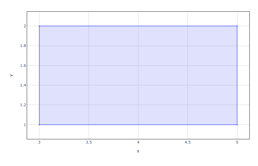
Plotting a Single Time Step#
Rather than animating all time steps in the polygon file, we might be interested in
plotting a specific time step. This can be easily accomplished by first accessing
the desired time step through the mahautils.multics.PolygonFile.polygon_data
property, and then using the mahautils.shapes.Layer.plot() method to plot
the geometry for the given time step.
For instance, suppose we want to plot the geometry at \(t = 2\ ms\).
>>> polygon_file.polygon_data[2].plot()
This should open a browser and display a figure similar to:
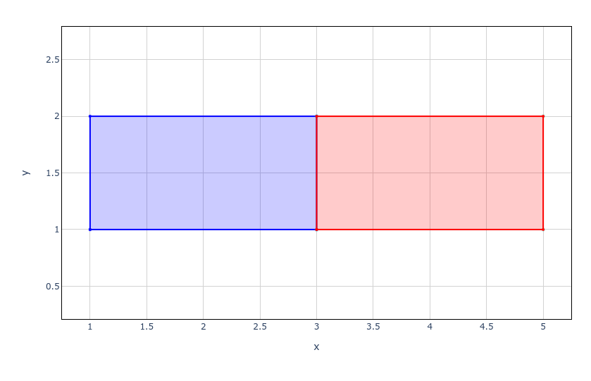
Using Plotly figures, it is possible to create much more advanced figures. For example, if we wanted to plot the polygon file geometry at \(t = 0\ ms\) and \(t = 2\ ms\) on the same plot, we could use the following commands:
>>> # Make the layers for each time step different colors
>>> polygon_file.polygon_data[0].color = 'blue'
>>> polygon_file.polygon_data[2].color = 'red'
>>> # Use "return_fig=True" to return the figure so we can modify it later
>>> fig = polygon_file.polygon_data[0].plot(show=False, return_fig=True)
>>> # Append the layer for a second time step to the figure
>>> fig = polygon_file.polygon_data[2].plot(figure=fig, show=False, return_fig=True)
>>> # Display the figure
>>> fig.show()
The result should look similar to this, where the polygon data for \(t = 0\ ms\) is blue and the data for \(t = 2\ ms\) is red: