Polygon File Format#
Maha Multics “polygon files” are used to store data about a set of polygons whose vertices may change position over time.
Applications#
One of the most common use cases for polygon files is when defining boundary conditions in lubricating films. Often, there are known pressures in certain geometric regions of the film (for instance, in the inlet and outlet ports), and it is necessary to communicate these geometric conditions to the solver. A polygon file can be a convenient way to provide this boundary condition.
Sample Application: Axial Piston Pump
Suppose that you are simulating an axial piston pump, and you want to model the cylinder block-valve plate interface.
In this interface, three boundary conditions are of interest, illustrated by the figure below. Note that the geometry in the figure is not representative of any real pump; it is for illustration purposes only. Additionally, while axial piston pumps typically have multiple displacement chambers, for simplicity only a single displacement chamber is shown in the figure.
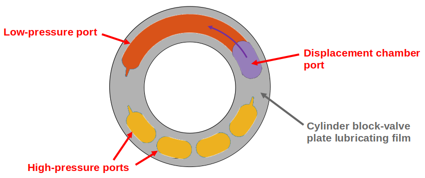
As seen in the figure above, three boundary conditions must be specified by defining polygon-shaped regions:
Low-pressure port (shown in orange): This port can have arbitrary shape, so its location must be specified using a polygon with an arbitrary number of vertices.
High-pressure ports (shown in yellow): These ports can have arbitrary shape, and since the high-pressure side of the valve plate in axial piston pumps typically has multiple ports separated by ribs for structural support, a union of disjoint polygons must be computed to accurately represent this boundary condition.
Displacement chamber port (shown in purple): The displacement chamber port pressure is typically calculated separately from solving the partial differential equations (PDEs) governing the film; thus, this port pressure can be considered a boundary condition, like the high- and low-pressure ports. An additional challenge is that this is a moving boundary condition, as the displacement chambers move following the rotation of the pump shaft (indicated by the purple arrow in the figure).
Of course, boundary conditions must also be defined on the inner and outer radii of the lubricating film, but these don’t need to be specified as arbitrary polygons, so they will not be discussed here.
Once we have defined the shapes of each of these three ports as polygons at each time step of the simulation, we can apply a constant-pressure boundary condition to each polygon region and use this as a boundary condition to solve the governing PDEs in the film. The polygon file discussed on this page addresses provides a data format that supports these needs.
Definitions#
Polygon
As discussed by Wolfram MathWorld, there is no universally-accepted definition of a polygon. The Maha Multics software uses a combination of elements of different definitions from multiple sources.
In general terms, the Maha Multics software defines a polygon as a closed, two-dimensional (2D) region bounded by a series of connected line segments that may or may not not intersect themselves.
Put another way, a polygon can be considered the closed 2D region bounded by line segments connecting a cyclical series of points in order, where the boundary never intersects itself.
Point-in-Polygon Problem
A point-in-polygon problem is a geometric problem attempting to determine whether a given point is inside or outside a (possibly self-intersection) polygon.
There are a number of algorithms that have been proposed for solving the point-in-polygon problem. The Maha Multics software uses the winding number algorithm.
For more detail on the point-in-polygon and winding number algorithm, refer to this paper.
Enclosed vs. Inside
This terminology is specific to the MahaUtils project and documentation.
The key purpose of Maha Multics polygon files is to determine whether points are considered “enclosed by” or within a given region of space (typically, so a boundary condition can be applied in these regions). The term enclosed by is used in this documentation to consider such regions.
The term inside is a more general mathematical term, commonly characterizing a mathematical problem in determining which points fall inside the perimeter of a polygon. The term “inside” will be used throughout this page in reference to the mathematical process (e.g., using algorithms such as winding number or ray casting) of solving the point-in-polygon problem.
File Format#
A polygon file stores the \(x\)- and \(y\)-coordinates of one or more polygons, at one or more instants in time. The purpose of the file is to store whether a point is “enclosed by” the polygon(s) at a specific point in time. In the event there are multiple polygons, there are several options for specifying how to define “enclosed,” as will be discussed below.
Warning
As explained below, the term “time” is used loosely with polygon files. The
measure of time does not necessarily need to be “physical time” (i.e.,
measured in seconds). Rather, it could be “time” measured as, for example,
the rotation angle of a pump shaft (in which case [TIME_UNIT] might be
degrees).
General Format#
There are two primary parts of a polygon file: (1) the header and (2) the polygon coordinates. The header lines in the files below are highlighted to distinguish the two parts of the file.
The standard format of a full polygon file is shown below. It can seem confusing at first, so if you aren’t sure about the format, skip to the later sections in which the format is broken down in more detail. The format is slightly different if storing one instant in time or multiple instants, and each is described under the tabs below.
 11 [Np] [POLYGON_MERGE_METHOD]
 2[NUM_COORD_1] [ENCLOSED_CONV_1]  # <-- polygon 1
 3[X_COORDINATE_UNIT]: [X_1] [X_2] ... [X_{NUM_COORD_1}]
 4[Y_COORDINATE_UNIT]: [Y_1] [Y_2] ... [Y_{NUM_COORD_1}]
 5[NUM_COORD_2] [ENCLOSED_CONV_2]  # <-- polygon 2
 6[X_COORDINATE_UNIT]: [X_1] [X_2] ... [X_{NUM_COORD_2}]
 7[Y_COORDINATE_UNIT]: [Y_1] [Y_2] ... [Y_{NUM_COORD_2}]
 8...
 9[NUM_COORD_j] [ENCLOSED_CONV_j]  # <-- polygon j
10[X_COORDINATE_UNIT]: [X_1] [X_2] ... [X_{NUM_COORD_j}]
11[Y_COORDINATE_UNIT]: [Y_1] [Y_2] ... [Y_{NUM_COORD_j}]
12...
13[NUM_COORD_Np] [ENCLOSED_CONV_Np]  # <-- polygon NUM_POLYGONS
14[X_COORDINATE_UNIT]: [X_1] [X_2] ... [X_{NUM_COORD_Np}]
15[Y_COORDINATE_UNIT]: [Y_1] [Y_2] ... [Y_{NUM_COORD_Np}]
 1[Nt] [Np] [POLYGON_MERGE_METHOD]
 2[TIME_UNIT]: [TIME_BEGIN] [TIME_STEP] [TIME_EXTRAP_METHOD]
 3[NUM_COORD_1_1] [ENCLOSED_CONV_1_1]  # <-- time step 1, polygon 1
 4[X_COORDINATE_UNIT]: [X_1] [X_2] ... [X_{NUM_COORD_1_1}]
 5[Y_COORDINATE_UNIT]: [Y_1] [Y_2] ... [Y_{NUM_COORD_1_1}]
 6[NUM_COORD_1_2] [ENCLOSED_CONV_1_2]  # <-- time step 1, polygon 2
 7[X_COORDINATE_UNIT]: [X_1] [X_2] ... [X_{NUM_COORD_1_2}]
 8[Y_COORDINATE_UNIT]: [Y_1] [Y_2] ... [Y_{NUM_COORD_1_2}]
 9...
10[NUM_COORD_1_Np] [ENCLOSED_CONV_1_Np]  # <-- time step 1, polygon NUM_POLYGONS
11[X_COORDINATE_UNIT]: [X_1] [X_2] ... [X_{NUM_COORD_1_Np}]
12[Y_COORDINATE_UNIT]: [Y_1] [Y_2] ... [Y_{NUM_COORD_1_Np}]
13[NUM_COORD_2_1] [ENCLOSED_CONV_2_1]  # <-- time step 2, polygon 1
14[X_COORDINATE_UNIT]: [X_1] [X_2] ... [X_{NUM_COORD_2_1}]
15[Y_COORDINATE_UNIT]: [Y_1] [Y_2] ... [Y_{NUM_COORD_2_1}]
16...
17[NUM_COORD_i_j] [ENCLOSED_CONV_i_j]  # <-- time step i, polygon j
18[X_COORDINATE_UNIT]: [X_1] [X_2] ... [X_{NUM_COORD_i_j}]
19[Y_COORDINATE_UNIT]: [Y_1] [Y_2] ... [Y_{NUM_COORD_i_j}]
20...
21[NUM_COORD_Nt_Np] [ENCLOSED_CONV_Nt_Np]  # <-- time step NUM_TIME_STEPS, polygon NUM_POLYGONS
22[X_COORDINATE_UNIT]: [X_1] [X_2] ... [X_{NUM_COORD_Nt_Np}]
23[Y_COORDINATE_UNIT]: [Y_1] [Y_2] ... [Y_{NUM_COORD_Nt_Np}]
Note that the numbers on the left-hand side are line numbers, and they are not part of the file.
Section 1: Header#
The header contains metadata about the polygon file, formatted as follows:
11 [Np] [POLYGON_MERGE_METHOD]
1[Nt] [Np] [POLYGON_MERGE_METHOD]
2[TIME_UNIT]: [TIME_BEGIN] [TIME_STEP] [TIME_EXTRAP_METHOD]
All parameters must be whitespace-separated.
Header Parameters for All Polygon Files#
These parameters should be included in all polygon files.
[Nt]: Number of Time Steps
The number of time steps in the file. Note that for files with a single
time step, Nt must be 1 (as shown in the code block above).
Must be an integer greater than or equal to 1.
[Np]: Number of Polygons per Time Step
The number of polygons per time step in the file, which must be the same for all time steps.
Must be an integer greater than or equal to 1.
Important
The Maha Multics software requires that the number of polygons is the same for all time steps. This is an internal limitation of the software.
[POLYGON_MERGE_METHOD]: Method for Combining Disjoint Polygons
In the event that there are multiple polygons per time step (i.e., Np > 1),
there are a variety of ways they could be combined. We might want to know
whether a point is enclosed by of all of the specified polygons, or any of
them, as a few examples.
There are three supported options for combining multiple disjoint polygons:
|
Description |
|---|---|
|
If a point is considered “enclosed by” of the union of polygons in the
file if it is enclosed by of any of the |
|
If a point is considered “enclosed by” of the union of polygons in the
file if it is enclosed by of all of the |
|
If a point is considered “enclosed by” of the union of polygons in the
file if it is enclosed by of exactly one of the |
Note that whether a point is enclosed by of each of the Np polygons will
be defined by the ENCLOSED_CONV parameter, discussed in the
Section 2: Polygon Coordinates section.
This parameters is only relevant for polygon files in which Np > 1
but a value should be included in all polygon files (if Np = 1, this
parameter is simply ignored).
Note
The same [POLYGON_MERGE_METHOD] must be used for all time steps. This
is a limitation hard-coded in the Maha Multics software.
Header Parameters for Files with Multiple Time Steps#
These parameters should be included only for polygon files multiple time steps (Nt > 1).
[TIME_UNIT]: Time Unit
A string describing the units in which the [TIME_BEGIN] and [TIME_STEP]
parameters are defined.
Note
Recall that the Maha Multics software uses “time” loosely, and the “time” can also be defined in terms of quantities such as “degrees of rotation of the pump shaft” or similar.
[TIME_BEGIN]: Initial Time
An integer or decimal number specifying the time for the first set of polygons stored in the file.
[TIME_STEP]: Constant Time Step
Type: Floating-point number
Restrictions: Must be a real number greater than 0
An integer or decimal number specifying the time step between each of
the [NUM_POLYGONS] specified polygons.
Important
The Maha Multics software requires that the time step is constant. This is an internal limitation of the software.
[TIME_EXTRAP_METHOD]: Extrapolation for Time Values
The parameters [NUM_TIME_STEPS], [TIME_BEGIN], and [TIME_STEP]
specify a range of times over which polygons will be provided; let us
denote this range \(t \in [t_{min}, t_{max}]\). This poses an
issue: what should be done if the time \(t\) falls outside this range?
It is not straightforward to “interpolate” or “extrapolate” polygons, since they can have an arbitrary number of coordinates that change in arbitrary ways each time step. Therefore, if \(t\) falls outside \([t_{min}, t_{max}]\), it must be “rescaled” to fall in this range.
Two options are provided for this “rescaling,” described below:
|
Description |
|---|---|
0 or 2 (saturation) |
When reading data from the polygon file, if \(t \lt t_{min}\), it is rescaled by \(t = t_{min}\), and if \(t \gt t_{max}\), it is rescaled by \(t = t_{max}\). |
3 (periodic) |
Assumes that the polygon data are periodic with period
\(t_{min} - t_{max} + \Delta t\), where \(\Delta t\) represents
|
Warning
If using the periodic approximation method (3), notice that you should not include both endpoints in the lookup table (otherwise, the period would be \(t_{max} - t_{min}\), not \(t_{max} - t_{min} + \Delta t\)).
For example, suppose your time variable is a cycle that repeats every rotation (\(360^\circ\)) and you are defining polygons in your polygon file every \(1^\circ\). In this case, your polygon file should include data for the following angles: \(0^\circ, 1^\circ, 2^\circ, ..., 358^\circ, 359^\circ\).
Section 2: Polygon Coordinates#
This section contains the \(x\)- and \(y\)-coordinates for all polygons in the file, for every time step. The general structure for specifying these points (for a single polygon) is shown below:
[NUM_COORD] [ENCLOSED_CONV]
[X_COORDINATE_UNIT]: [X_1] [X_2] ... [X_{NUM_COORD}]
[Y_COORDINATE_UNIT]: [Y_1] [Y_2] ... [Y_{NUM_COORD}]
Note that Section 2 of a polygon file typically contains a number of code blocks similar to above. However, each has the same format, so only a single such block will be discussed here. To see how to use multiple such blocks, refer to the Examples section.
The following parameters must be included in this section:
[NUM_COORD]: Number of Points on Polygon Perimeter
The number of \(x\)- and \(y\)-coordinates specifying the polygon perimeter.
Must be an integer greater than or equal to 3.
Note
This information is technically redundant since the coordinates themselves are given. This is an internal limitation of the Maha Multics software.
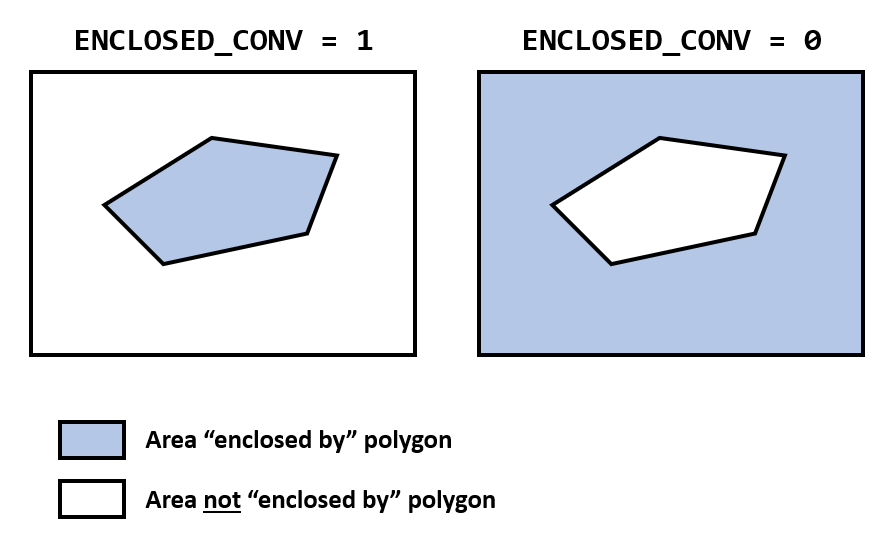
[ENCLOSED_CONV]: How to Define Area “Enclosed By” the Polygon
This input clarifies, for every polygon, what area is considered to be “enclosed by” the polygon. Particularly for polygons with self-intersecting edges, it can be difficult to intuitively and visually assess which regions are “enclosed by” the polygon.
The Maha Multics software uses the winding number algorithm to determine which points are
inside a polygon. If these points are to be considered “enclosed by” the polygon
for the purposes of the polygon file definition, then set ENCLOSED_CONV to 1.
To reverse this convention, set ENCLOSED_CONV to 0.
The figure and table below clarify these conventions.
|
Description |
|---|---|
1 |
Points “inside” the polygon based on the winding number algorithm are considered enclosed by the polygon in the Maha Multics polygon file |
0 |
Points “inside” the polygon based on the winding number algorithm are considered not enclosed by the polygon in the Maha Multics polygon file |
Note
This value should almost always be 1 for simple polygons. It is primarily included for handling self-intersecting polygons and for backwards
compatibility of the Maha Multics software.
[X_COORDINATE_UNIT] and [Y_COORDINATE_UNIT]: Units
These parameters specify the units for the \(x\)- and \(y\)-coordinates specified on the same line as the unit.
[X_1], [Y_1], ..., [X_N], [Y_N]: Perimeter Coordinates
The \(x\)- and \(y\)-coordinates of the polygon perimeter must be
provided on two separate lines. All coordinates should be whitespace-separated,
and there should be a total of NUM_COORD \(x\)-coordinates and
NUM_COORD \(y\)-coordinates.
Examples#
Single, Stationary Polygon#
Consider perhaps the simplest possible polygon file: a single polygon, at a single time step. Suppose that we want to describe a rectangle with vertices \((1, 0)\), \((5, 0)\), \((5, 2.5)\), \((1, 2.5)\).
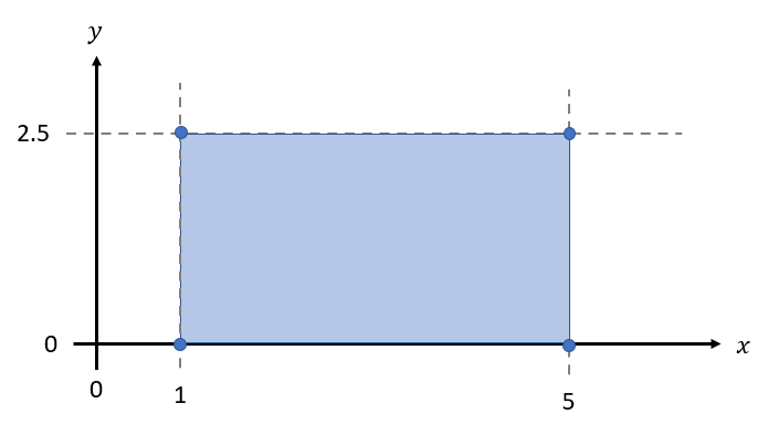
In this case, there is one time step (Nt = 1) and a single polygon (Np = 1).
Since there is only one polygon, POLYGON_MERGE_METHOD is not relevant (we’ll
set it to 0 for this example). We’ll assume that all coordinates are in units of
m and that the area inside the rectangle based on the winding number algorithm is
to be considered “enclosed by” the polygon (ENCLOSED_CONV = 1).
Taken together, these parameters result in the following polygon file:
1 1 0
4 1
m: 1  5  5    1
m: 0  0  2.5  2.5
Multiple, Stationary Polygons#
Let’s extend the previous example to a union of two polygons:
A rectangle with vertices \((1, 0)\), \((5, 0)\), \((5, 2.5)\), \((1, 2.5)\)
A triangle with vertices \((5, 0)\), \((5, 2.5)\), \((7.5, 0)\)
Visually, this union is the following pentagon:
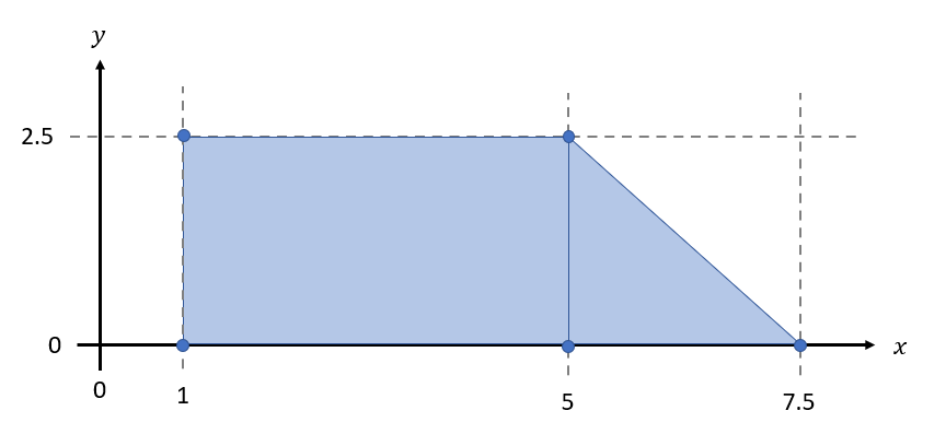
In this example, there is one time step (Nt = 1) and two polygons (Np = 2). Since
we want to consider the area enclosed by either of the two polygons as enclosed by their
union, POLYGON_MERGE_METHOD should be 0. We’ll assume that all coordinates are in
units of cm and that the area inside both the rectangle and triangle based on the
winding number algorithm is considered enclosed by the polygon union (ENCLOSED_CONV = 1).
Taken together, these parameters result in the following polygon file:
1 2 0
4 1
cm: 1  5  5    1
cm: 0  0  2.5  2.5
3 1
cm: 5  5    7.5
cm: 0  2.5  0
Single, Moving Polygon#
Finally, consider a case in which a polygon is moving. This is particularly applicable to fluid power applications, as this may reflect the moving boundary conditions in lubricating films.
As a simple example, consider a rectangular polygon that moves between \(t = 0\ ms\) and \(t = 2\ ms\) as shown below.
Thus, the rectangle has the following vertices at each time step:
\(t\) |
Vertices |
|---|---|
\(0\ ms\) |
\((1, 1)\), \((3, 1)\), \((3, 2)\), \((1, 2)\) |
\(1\ ms\) |
\((2, 1)\), \((4, 1)\), \((4, 2)\), \((2, 2)\) |
\(2\ ms\) |
\((3, 1)\), \((5, 1)\), \((5, 2)\), \((3, 2)\) |
In this case, there are three time steps (Nt = 3) and one polygon (Np = 1).
Since there is only one polygon, POLYGON_MERGE_METHOD is not relevant (we’ll
set it to 0 for this example). The units of time are ms ([TIME_UNITS] = ms),
and since the time begins at zero and advances in \(1\ ms\) increments,
[TIME_BEGIN] = 0 and [TIME_STEP] = 1. Assuming that we want to use
“saturation” for time extrapolation, [TIME_EXTRAP_METHOD] = 0.
Based on the parameters described above and assuming that the coordinates are in
units of ft, these parameters result in the following polygon file:
3 1 0
ms: 0 1 0
4 1
cm: 1  3  3  1
cm: 1  1  2  2
4 1
cm: 2  4  4  2
cm: 1  1  2  2
4 1
cm: 3  5  5  3
cm: 1  1  2  2
Comments, Whitespace, and Line Endings#
Comments should not be used in polygon files.
Items denoted “whitespace-separated” may be separated by either spaces or tab (
\t) characters.Blank lines may be included but are not recommended.
On Linux and MacOS, LF line endings (
\n) must be used. On Windows, either LF (\n) or CRLF (\r\n) line endings may be used.