SimViewer GUI
The SimViewer graphical user interface (GUI) is a tool for quickly plotting and visualizing Maha Multics simulation results files. It is built on Plotly Dash and runs in a web browser, so it is compatible with most operating systems.
Most of the features of the SimViewer tool are self-explanatory, so this guide will describe everything in detail, instead highlighting key features.
Note
Try it out! As you follow along this guide, feel free to use these sample
simulation results files to try out the features:
sim_results_underdamped.txt,
sim_results_overdamped.txt
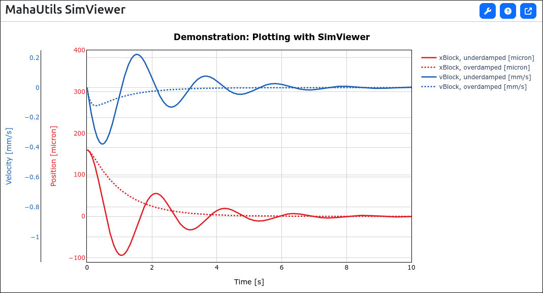
These files are hypothetical simulations illustrating typical underdamped and overdamped transient responses.
Motivation
SimViewer is designed to assist in quick exploration of simulation results data. Several priorities were considered when designing the tool:
The general use case is for Maha Multics numerical simulations, where the simulation generates a number of different properties (body positions, friction forces, etc.) that are all a function of time (or some measure of time, such as shaft position). Therefore, it is necessary to plot multiple variables, possibly with very different scales, as a function of a single variable (time).
Often, similar plots need to be generated for multiple simulations. For instance, one might be experimenting with different mesh sizes and need to generate the same plots of pressure and film thickness. SimViewer provides an option to save plot configuration files so that plots can be rapidly generated.
Sometimes, results from multiple simulations need to be compared. SimViewer allows users to load and compare an arbitrary number of simulation results (assuming your system has enough memory to support it).
Launching SimViewer
Installation
Follow the installation instructions to install the MahaUtils package on your computer with pip. Once this package is installed, SimViewer will be available.
Alternatively, if you just want to try out SimViewer or for any reason cannot install the package on your system, you can use GitHub Codespaces to test the GUI. Note that a GitHub account is required.
Command-Line Options
SimViewer is a graphical tool, but it must be launched from the command line. To run SimViewer, simply open a terminal (activating your virtual environment, if applicable), and run:
SimViewer
Note that there are several optional command-line arguments. To view these options, run:
SimViewer --help
One important option to notice is --port. SimViewer runs as a web app, and
this argument sets the port on which the app is served. For instance, to
launch a SimViewer instance on port 9876, run:
SimViewer --port 9876
Important
If running multiple SimViewer instances, be sure to use a different port for each instance.
Configuring Plot Settings
Almost all plot configuration settings can be edited through the configuration pane, which can be opened using the icon in the top-right corner:

This should open a panel that contains a number of options for managing data and plot formatting:
Loading Data
The first step when using SimViewer is to load Maha Multics simulation results files to plot. This can be accomplished on the “Data Files” tab:

Either drag-and-drop your file, or click the dotted box and browse to your file. When uploading files, you will be asked to enter a name for the file. This should be a short identifier that you can use later to select which file to plot data from, so choose a short but descriptive name.
The “Current Files” section of the “Data Files” tab lists all currently loaded data files and offers the following options:
Enabled switches: These represent a “global” on/off switch that will show or hide all data series associated with a file.
Delete buttons: Deletes the simulation results file.
Plotting Data
The key principle behind SimViewer is that when plotting Maha Multics simulation results, it is typical that there is a single independent variable (time, or some measure of time such as shaft rotation angle) and multiple dependent variables. In this documentation, the independent variable is assumed to be plotted on the (horizontal) \(x\)-axis, and the dependent variables – referred to as data series – are plotted on the (vertical) \(y\)-axis. In addition, SimViewer offers the capacity to create multiple \(y\)-axes to group data series.
Plot Configuration: \(x\)-axis
The first step when plotting simulation results data is to select the independent variable. This can be performed on the “X-Axis” tab:

Because we assume that there is a single independent (time) variable, the x-axis variable can be selected from any simulation results variable that is present in all uploaded simulation results files.
Notice that it is required to set units for the independent variable. Any units defined in the default unit converter can be chosen; unit conversions are performed automatically.
Plot Configuration: \(y\)-axes
Next, we need to select which data series (i.e., dependent variables) to plot. These options can be selected on the “Y-Axes” tab:
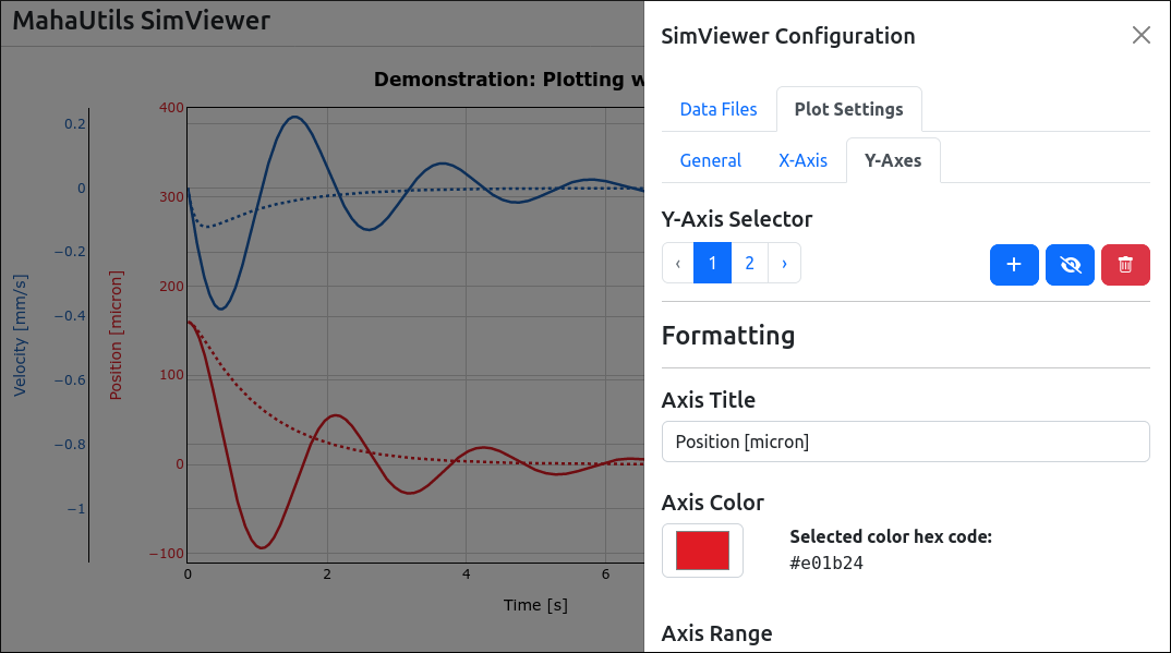
As mentioned previously, it is possible to create multiple \(y\)-axes. These can be managed under the “Y-Axis Selector” section – here, you can switch between \(y\)-axes, create/delete axes, and hide/show an axis. Additionally, you can set a number of formatting options, such as the title for the \(y\)-axis and a color (to make it visually easier to identify).
Each \(y\)-axis can plot one or more data series (each of which can be selected from any simulation results file). To manage data series for a particular \(y\)-axis, select the axis under the “Y-Axis Selector” section, and then scroll down to the “Data Series Configuration” section:
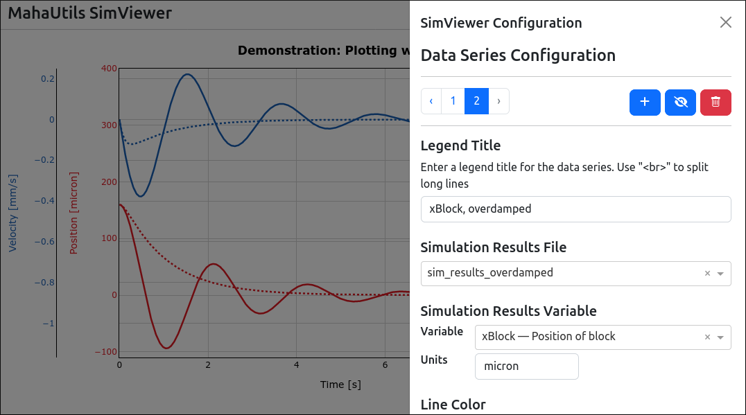
In this section, you can add any desired data series to the \(y\)-axis. Simply select the file from which the data series should be obtained, and which variable and units with which to plot the data. Any units defined in the default unit converter can be chosen; unit conversions are performed automatically.
Similar to the \(y\)-axis selection, you can switch between and manage (add, delete, hide, show) data series using the controls in the “Data Series Configuration” section. In addition, formatting options are available to change line colors, width, and style.
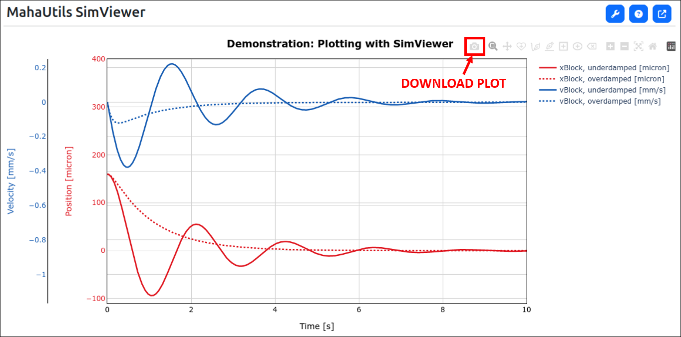
Downloading Plots
Once you’ve generated a beautiful SimViewer plot, you may be wondering…how can I download it to frame and hang on my wall?
We’ve got you covered! Just click the “download plot” button:
You can even customize the file format, aspect ratio, and image sizing under the “General” settings tab:

Saving Plot Configuration
Often, when plotting simulation results, the same plots are created repeatedly. For instance, you might be developing code for a simulation and want to check how the results compare after each iteration. Rather than having to manually create new plots each time, SimViewer provides a means to store your plot settings and generate desired figures with the click of a button.
Exporting Plot Configuration Settings
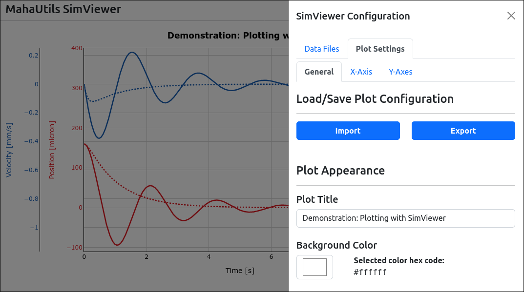
Once you have configured your plot with all desired options, navigate to the “General” tab and click the “Export” button:
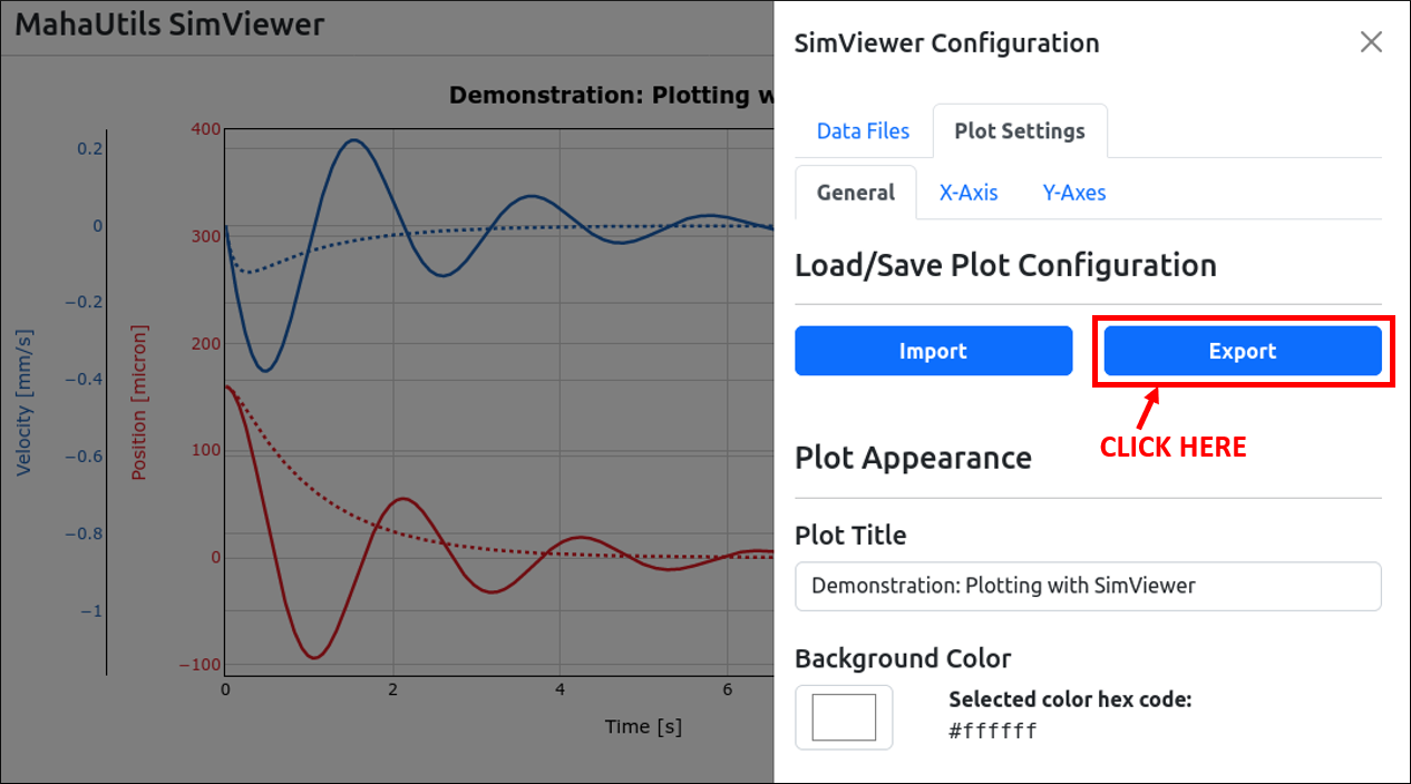
This will save all plot configuration settings to a JSON file.
Importing Plot Configuration Settings
Later, if you want to create the same set of plots with SimViewer, follow these steps to restore the same plot settings using this configuration file:
Launch SimViewer and import your simulation results files (under the “Data Files” tab), making sure to label the files with the same names as you did originally when creating the JSON configuration file.
Navigate to the “General” tab and select “Import” to load your JSON configuration file. (tip: you can also simply drag-and-drop your JSON configuration file onto the “Import” button)
The plot should automatically be updated and restore your previous configuration.
Important
Be sure to upload your simulation results files (under the “Data Files” tab) before you import the JSON configuration file. Additionally, make sure that when loading the simulation results files, you choose the same names as you did when originally creating the JSON configuration file.
Note that you can also use this JSON configuration file to generate plots of the same \(x\)- and \(y\)-variables from different Maha Multics simulation results files – just use the same name when uploading the files.